What is PCA Color Augmentation?
Author: Addie Ira Borja Parico.
Data augmentation is the artificial enlargment of the dataset to reduce overfitting on the image data during training. The easiest and most common method to perform data augmentation is to use transformations that preserve the labels. One example is PCA Color Augmentation.
PCA Color Augmentation (also called Fancy PCA) alters the intensities of the RGB channels along the natural variations of the images, denoted by the principal components of the pixel colors (Bargoti & Underwood, 2016). It performs Principal Components Analysis on the color channels, thus, given the name Fancy PCA.
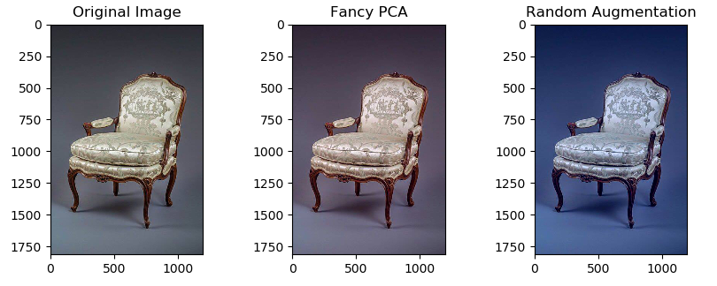
(Image Source: https://pixelatedbrian.github.io/2018-04-29-fancy_pca/)
The figure above shows an example of how Fancy PCA looks very natural compared to random changes in the RGB intensities. To make the intensity change more obvious to the naked eye, augmentation in this example was magnified by ~1000x.
"What do I need to know before learning Fancy PCA?"
If you have a good foundation in linear algebra, you will be able to fully grasp the algorithm of fancy PCA.
If you are a beginner both to linear algebra and fancy PCA, here's a playlist of Youtube videos to teach you about the fundamentals of linear algebra.
After that, read about principal component analysis (PCA). Or you can watch this step-by-step video about PCA.
How Fancy PCA works
This method is based on the study by Krizhevsky, Sutskever & Hinton (2012), the proponents of AlexNet.
Specifically, Principal Component Analysis is performed on the set of RGB pixel values throughout the image dataset. To each image, multiples of the found principal components are added, with magnitudes proportional to the corresponding eigenvalues times a random variable drawn from a Gaussian distribution with mean=0 and standard deviation=0.1.
Therefore to each RGB image pixel $I_{xy}= [I_{xy}^R,I_{xy}^G,I_{xy}^B]^T$ the following quantity is added:
$[p_1,p_2,p_3][\alpha_1\lambda_1,\alpha_2\lambda_2,\alpha_3\lambda_3]$
where $p_1$ and $\lambda_i$ are $i$th eigenvector and eigenvalue of the 3 × 3 covariance matrix of RGB pixel values, respectively, and $\alpha_i$ is the aforementioned random variable. Each $\alpha_i$ is drawn only once for all the pixels of a particular training image until that image is used for training again, at which point it is re-drawn.
Step-by-step algorithm of Fancy PCA
This algorithm is mainly based on this Python code for Fancy PCA (with few modifications). I used numpy and PIL libraries.
Step 1. Load the image(s) as a numpy array with (h, w, rgb) shape as integers between 0 to 255
from numpy import asarray
from PIL import Image

im = Image.open('image.jpg') #load image.jpg
i_a = asarray(im) #convert image to array
Step 2. Convert the range of pixel values from 0-255 to 0-1
i_a = i_a / 255.0Step 3. Flatten the image to columns of RGB (3 columns)
Flattening the images merges all the layers (in this case, RGB layers) into one column each color channel.
img_rs = i_a.reshape(-1, 3)Step 4. Centering the pixels around their mean (for more info, click here)
img_centered = img_rs - np.mean(img_rs, axis=0)Step 5. Calculate the 3x3 covariance matrix using numpy.cov. The parameter rowvar is set as False because each column represents a variable, while rows contain the values.
img_cov = np.cov(img_centered, rowvar=False)Step 6. Calculate the eigenvalues (3x1 matrix) and eigenvectors (3x3 matrix) of the 3 x3 covariance matrix using numpy.linalg.eigh
eig_vals, eig_vecs = np.linalg.eigh(img_cov)Then, sort the eigenvalues and eigenvectors
sort_perm = eig_vals[::-1].argsort()
eig_vals[::-1].sort()
eig_vecs = eig_vecs[:, sort_perm]
After that, you will finally get eigenvector matrix [p1, p2, p3] as:
m1 = np.column_stack((eig_vecs))Step 7. Get a 3x1 matrix of eigenvalues multipled by a random variable drawn from a Gaussian distribution with mean=0 and sd=0.1 using numpy.random.normal
One thing to note, according to Krizhevsky, Sutskever & Hinton (2012), is that the alpha should only be drawn once per augmentation (not once per channel)
m2 = np.zeros((3, 1))
alpha = np.random.normal(0, 0.1)
Step 8. Create and add the vector (add_vect) that we're going to add to each pixel
m2[:, 0] = alpha * eig_vals[:]
add_vect = np.matrix(m1) * np.matrix(m2)

for idx in range(3):   # RGB
    orig_img[..., idx] += add_vect[idx]
Step 9. Convert the range of arrays from 0-1 to 0-255 (u-int8)
orig_img = np.clip(orig_img, 0.0, 255.0)
orig_img = orig_img.astype(np.uint8)

return orig_img
Step 10. Convert the array of the augmented image back to jpg using Image.fromarray
final_img = Image.fromarray(orig_img)Fancy PCA on batch of images
The code below is to perform fancy PCA to a batch of images in a folder to another destination folder. Try editing path, path2 and path3 to test your own image.
# Import required libraries
from numpy import asarray
import argparse
import fancy_pca
from PIL import Image
import os
import glob
import numpy as np


# Load multiple images
image_list = []
fname_list = []
path = '/content/drive/My Drive/images/orig/lori.jpg' # path of the original image dataset.
path2 = '/content/drive/My Drive/images/orig/' # path of the original dataset folder

# Load images and put them in a list (image_list)
for infile in glob.glob(path):
    im = Image.open(infile)
    image_list.append(im)

# Extract the names of the files and put them in a list (fname_list)
base = os.listdir(path2)
for f in base:
    fname = os.path.splitext(f)
    fname_list.append(fname[0])
    print("Loading",infile)
    print(len(image_list)," images has loaded.")


# Convert images to numpy arrays
array_list =[]
n=1
for i in image_list:
    i_a = asarray(i)
    array_list.append(i_a)
    print("Image", n, ": Conversion successful.")
    n+=1
print("Array of original image: ", i_a) #To see the array

print("Conversion successful")
print(type(i_a), i_a.shape)

# Perform the PCA color augmentation
n=1
aug_list=[]
for a in array_list:
    augmented = fancy_pca.fancy_pca(a)
    aug_list.append(a)
    print("Array",n, ":Augmentation successful")
    n += 1
print("Array of PCA augmented image: ", augmented) #To see the array

# Convert Fancy PCA result back to PIL image
path3 = "/content/drive/My Drive/images/aug/" #path of the destination folder
idx=0
for aug in aug_list:
    i2 = Image.fromarray(aug)
    print(fname_list)
    while idx<= len(fname_list):
        print(str(fname_list[idx])+"_1.jpg")
        i2.save(path3+(str(fname_list[idx])+"_1.jpg"))
        break
    idx+=1
    print("Augmented image", idx, "saved.")
Literature Cited
- Bargoti, S., Underwood, J. (2016). Deep Fruit Detection in Orchards. Proceedings - IEEE International Conference on Robotics and Automation, 3626–3633. https://doi.org/10.1109/ICRA.2017.7989417
- Krizhevsky, A., Sutskever, I., Hinton, G. E. (2012). ImageNet classification with deep convolutional neural networks. In F. Pereira, C. J. C. Burges, L. Bottou, & K. Q. Weinberger (Eds.), Advances in neural information processing systems 25 (pp. 1097–1105). Curran Associates, Inc. Retrieved from https://papers.nips.cc/paper/4824-imagenet-classification-with-deep-convolutional-neural-networks.pdf